Anime shows - Longer titles yet shorter seasons

Motivation¶

In recent years, I’ve seen the titles of anime got so much longer. This is especially true for the Isekai genre, with titles packed with descriptive clauses and information, e.g. That Time I Got Reincarnated as a Slime.

Curious, I wanted to do some analysis on this. Other people have also looked at this by the way, to some extent. I wanted as comprehensive dataset as possible, since there are multiple databases out there but they may not be complete. Luckily, the Manami Project archives anime metadata, sourcing and combining from multiple known databases.

Takeaway¶

I was able to use this dataset, with most focus on anime TV series. Essentially, titles of anime series have really been getting longer, with tremendous increases within the past 5 years of so. This is generally true for ONA (Original Net Animation).
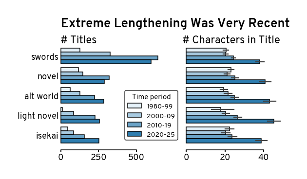
However, short anime, including movies, specials and OVA (Original Video Animation), show much more non-monotonic trends. Looking closely at the top 5 most recent anime tags (anime adpated from novels or have something about alternative worlds or swords), it really seems that the increases are extremely “explosive” in the past 5 years.

Additionally, I was also curious at the length of shows as well, as I was noticing anime getting shorter in terms of the number of episodes. It used to be that a season would be around 20 or 24 episodes at least, but recently it seems that a season lasts typically 12 or 13 episodes. This was observed by other people as well Looking quickly at this dataset, it seems that TV series have in fact gotten much shorter in terms of number of episodes per season, though interesting ONA, which used to be much shorter than TV, has been slowly approaching length.

Requirements¶

Data¶

The anime dataset is from manami-project/anime-offline-database, specifically the file anime-offline-database.jsonl.zst from version 2026-02. The dataset was downloaded on Jan 11, 2026. Since no collection was needed, it can be downloaded straight from the source.

Code¶

Source code: https://codeberg.org/penguinsfly/tv-mania/src/branch/main/anime-names.

The required dependencies are listed in requirements.txt in this folder of the respository.

Import packages & set configurations¶

import numpy as np
import pandas as pd
import networkx as nx

from matplotlib import (
    pyplot as plt,
    rcParams
)
import seaborn as sns

# plot configs
rcParams['font.family'] = 'Overpass Nerd Font'
rcParams['font.size'] = 18
rcParams['axes.titlesize'] = 20
rcParams['axes.labelsize'] = 18
rcParams['axes.linewidth'] = 1.5
rcParams['lines.linewidth'] = 1.5
rcParams['lines.markersize'] = 20
rcParams['patch.linewidth'] = 1.5
rcParams['xtick.labelsize'] = 18
rcParams['ytick.labelsize'] = 18
rcParams['xtick.major.width'] = 2
rcParams['xtick.minor.width'] = 2
rcParams['ytick.major.width'] = 2
rcParams['ytick.minor.width'] = 2
rcParams['savefig.dpi'] = 300
rcParams['savefig.transparent'] = False
rcParams['savefig.facecolor'] = 'white'
rcParams['savefig.format'] = 'svg'
rcParams['savefig.pad_inches'] = 0.5
rcParams['savefig.bbox'] = 'tight'

# modified from Vibrant Summer cmap: https://coolors.co/palette/ff595e-ffca3a-8ac926-1982c4-6a4c93
# type_cmap = dict(zip(
#     ['TV', 'ONA', 'MERGED',
#      'OVA', 'MOVIE', 'SPECIAL',],
#     sns.color_palette('Dark2', 6)
# ))

type_cmap = dict(zip(
    ['TV', 'ONA', 'MERGED',
     'OVA', 'MOVIE', 'SPECIAL',],
    ['#E94B50', '#E8B731', '#1982C4',
     '#8AC926', '#C8851A', '#6A4C93',]        
))

Load data¶

df = (
    pd.read_json(
        'anime-offline-database.jsonl.zst', 
        lines=True
    )
    .filter([
        'title', 'type', 'tags',
        'episodes', 'animeSeason',
        'sources', 'relatedAnime',
        'score',
    ])
    .dropna(
        subset=['title','animeSeason'],
        how='any', 
        ignore_index=True
    )
    .astype({'title': 'str'})
)

df['year'] = df.pop('animeSeason').apply(lambda x: x.get('year',None))

Limit to only titles between 1980 and 2025. And then compute the length of titles by number of characters or “words” (i.e. split by spaces).

df = (
    df
    # .query('type == "TV"')
    .query('type != "UNKNOWN"')
    .query('episodes > 0.0')
    .query('year >= 1980 and year <= 2025')  
    .dropna(subset='year', ignore_index=True)
    .astype({'year':'int'})
    .reset_index()
    .rename(columns={'index':'ID'})
)

df['num_chars'] = df['title'].apply(len)
df['num_words'] = df['title'].str.split().apply(len)

df

Merge titles¶

Some titles are related to each other, e.g. each season is an entry itself and there may be specials for a show.

Hence, I also wanted to look at the entire anime as a whole, and merge to the first existing entry, e.g. analyzing Attack on Titans as a whole when it was first released, rather than every single season separately.

max_cc_ids = 100 # some odd cc's may have been constructed
idf = pd.concat([
    (
        df.rename(columns={'sources':'source'})
        .filter(['ID','source'])
        .explode('source')
        .drop_duplicates()
        .dropna()
    ),
    (
        df.rename(columns={'relatedAnime':'source'})
        .filter(['ID','source'])
        .explode('source')
        .drop_duplicates()
        .dropna()
    ),
], ignore_index=True)

idf = idf.drop_duplicates(ignore_index=True)

G = nx.from_pandas_edgelist(idf, source='source', target='ID')
cc_df = pd.DataFrame([
    dict(
        cc = cc_id,
        ID = [xi for xi in x if isinstance(xi, int)]
    ) for cc_id, x in enumerate(nx.connected_components(G))
])
cc_df['size'] = cc_df['ID'].apply(len)
cc_df = (
    cc_df.query('size <= @max_cc_ids')
    .drop(columns='size')
    .reset_index(drop=True)
)
cc_df

Visualize title and anime length across time¶

Note that due to the low number of titles before 2000, relatively compared to after 2000, I grouped titles 1980-1999 into two decades.

vdf = df.melt(
    id_vars=['ID', 'year','type'],
    value_vars=['num_chars','num_words','episodes']
)

vdf = pd.concat([
    vdf,
    (
        cc_df
        .explode('ID')
        .merge(df, how='left')
        .sort_values(['cc','year'])
        .groupby('cc')
        .head(1)
        .melt(
            id_vars=['ID', 'year'],
            value_vars=['num_chars','num_words']
        )
        .assign(type='MERGED')
    ),
], ignore_index=True)

vdf = pd.concat([
    vdf,
    (
        vdf.groupby(['year','type'])
        ['ID'].nunique()
        .to_frame('value')
        .assign(variable='num_entries')
        .reset_index()
    ),
], ignore_index=True)    
    
vdf['vis_period'] = vdf['year'].apply(
    lambda x: (
        '1990-1999' if x < 2000 and x >= 1990 
        else '1980-1989' if x < 1990 
        else 'year' 
    )
) 

vdf['vis_year'] = vdf['year'].apply(
    lambda x:  (
        1997 if x < 2000 and x >= 1990 
        else 1994 if x < 1990 
        else x
    )
)

vdf['vis_block'] = vdf['type'].map({
    'TV': 'Long anime',
    'ONA': 'Long anime',
    'MERGED': 'Long anime',
    'OVA': 'Short anime',
    'MOVIE': 'Short anime',
    'SPECIAL': 'Short anime',
})

vis_label_maps = {
    'num_entries': '# Anime Titles', 
    'num_chars': '# Characters in Title',
    'num_words': '# Words in Title',
    'episodes': '# Episodes',
}
vdf['vis_label'] = vdf['variable'].map(vis_label_maps)

vdf

g = sns.relplot(
    vdf,
    x='vis_year',
    y='value',
    hue='type',
    hue_order=type_cmap.keys(),
    palette=type_cmap,
    err_kws=dict(alpha=0.2),
    col='vis_label',
    col_order=vis_label_maps.values(),
    row='vis_block',
    row_order=['Long anime','Short anime'],
    kind='line',
    size='vis_period',
    size_order=['1980-1989','1990-1999','year'],
    sizes=[1,1,1],
    marker='.',
    markersize=10,    
    markeredgecolor='none',
    facet_kws=dict(
        margin_titles=True,
        sharex=True,
        sharey=False,
    ),
    height=3.5,
    aspect=1.2,
    zorder=2,    
    # n_boot=20, # for quick debug
    legend=False, # flip to debug
)

g.set_titles(
    col_template='{col_name}',
    row_template='{row_name}',
    size=20,
)

[
    g.refline(
        x=xi,ls='--',
        c='.8' if xi != 2000 else '.1',
        lw=0.5 if xi != 2000 else 1
    ) 
    for xi in range(2000,2026,10)
]
plt.xticks([2000, 2010, 2020])

axes = g.axes.flat
axes[0].set_ylim([-1, 1100])
axes[1].set_ylim([0, 40])
axes[2].set_ylim([0, 8])
axes[3].set_ylim([0, 80])

axes[4].set_ylim([-1, 1100])
axes[5].set_ylim([0, 40])
axes[6].set_ylim([0, 8])
axes[7].set_ylim([0, 6])

[
    axes[3].axhline(y=yi,ls=':',c='.5') 
    for yi in [12,24]
]

legend_text_kws = dict(    

)

[
    axes[iax].text(
        x=2001, y=1000-200*i,
        s=t, color=type_cmap[t],
        fontsize=18, fontweight='bold',
        ha='left', va='top',
    ) 
    for iax, ts in [
        [0, ['MERGED','ONA','TV']], 
        [4, ['SPECIAL', 'MOVIE','OVA']]
    ]
    for i,t in enumerate(ts)
]

[ 
    axes[i].set_title(
        axes[i].get_title(),
        fontsize=24, y=1.05,
        ha='left', x=0
    )
    for i in range(4)
]
g.set_xlabels('Released Year')
g.set_ylabels('')

[
    axes[i].text(
        x=x,y=y,s=s,
        ha='center',va='bottom',
        fontsize=15, fontstyle='italic',
        rotation=90, color='.6',
    )
    for x, s in [(1994,'1980-89'),(1997,'1990-99')]
    for i, y in [
        (0,600),(4,600),
        (1,1),(5,1),
        (2,0.1),(6,0.1), 
        (3,30), (7,4),
    ]
]
g.fig.suptitle(
    'Anime TV Series Get Longer Names But Shorter Seasons',
    x=0.05, y=1.0, ha='left',
    fontweight='bold', fontsize=40,    
)

g.despine(trim=True,offset=2)
g.tight_layout(w_pad=3, h_pad=3)
plt.savefig('figures/trends.svg')
plt.savefig('figures/trends.png')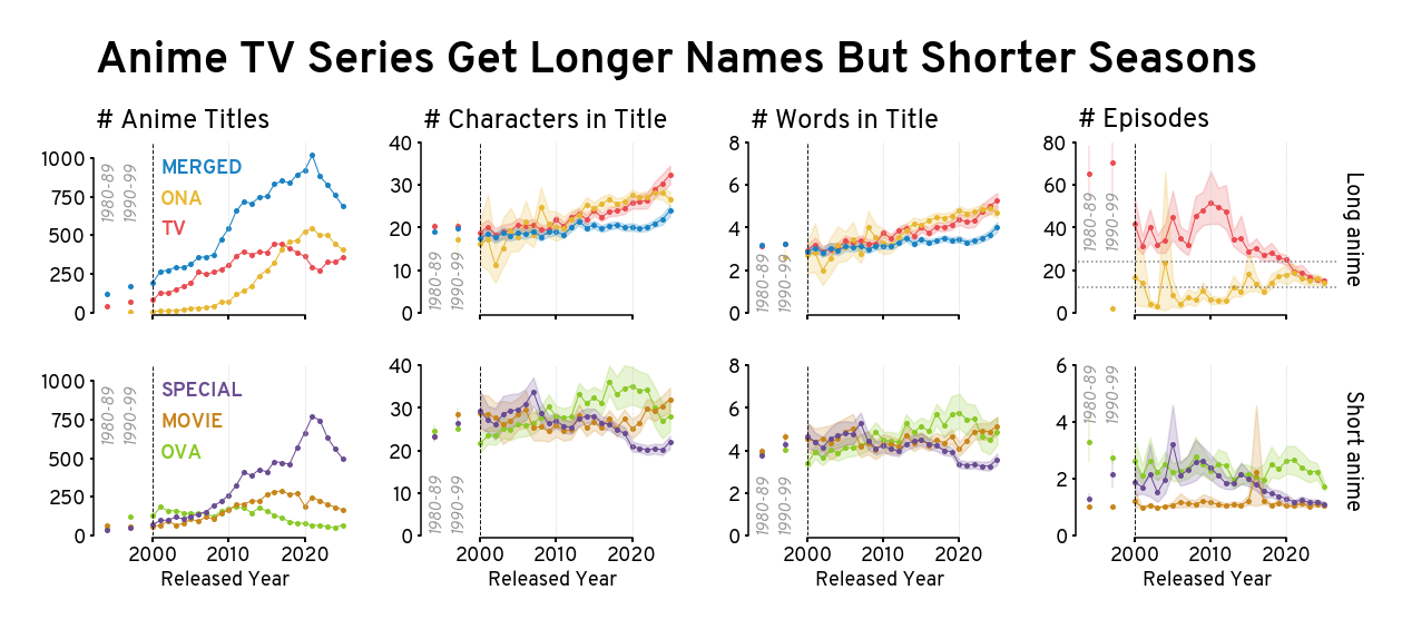

This supports the statements that anime generally have been getting much longer in terms of their names, especially after 2010 for TV. And even for merged entries, titles have also gotten longer, though showing most clearly in the last 5 years. It is interesting that for short anime in general have much more non-monotonic trends throughout the years.

And while titles have consistently gotten longer for long anime, it seems that their length, by episode number, has converging to some average below 20 episodes per season. The length for short anime either hasn’t changed much (movies and OVA) or shows a decrease trend to single-episode specials.

What are the top tags in terms of title length of TV?¶

Next, let’s explore the top tags per periods, in terms of their title length. And focus on TV only for simplicity. Additionally, let’s also look at their quality (i.e. mean ratings since the three score variables in the database are very correlated).

tags_df = (
    df
    .query('type == "TV"')
    .filter([
        'ID','title','tags', 
        'year', 'score', 
        'num_chars', 'num_words'
    ])
    .reset_index(drop=True)
)
tags_df['score'] = tags_df['score'].apply(
    lambda x: np.nan if not isinstance(x, dict) else
        x.get('arithmeticMean',np.nan)
)

tags_df['period'] = pd.cut(
    tags_df['year'],
    [1980,2000,2010,2020,2026],
    right=False
).apply(
    lambda x: f'{x.left}-{str(x.right-1)[2:]}'
)

tags_df

The median score (~7) will be used to delinate between low and high quality shows

med_tv_score = tags_df['score'].median()
med_tv_score

6.697499175427747

Additionally, just as a sanity fact there is no relationship between the quality of shows and their title lengths.

tags_df.groupby('period', observed=False)[['score','num_words']].corr()

renamed_tags = {
    # some manual renaming
    # this was actually done iteratively with the later cells        
    'science-fiction': 'scifi',
    'science fiction': 'scifi',
    'sci fi': 'scifi',
    'sci-fi': 'scifi',
    'swords & co': 'swords',
    'swordplay': 'swords',
    'sword': 'swords',
    'alternative world': 'alt world',
    'alternate world': 'alt world',
    'based on a visual novel': 'visual novel',
    'visual novels': 'visual novel',
    'based on a light novel': 'light novel',
    'based on a novel': 'novel',
    'based on a web novel': 'web novel',    
}

tags_adf = (
    tags_df
    .explode('tags')
    .rename(columns={'tags':'tag'})
    .dropna(subset='tag')
    .replace({'tag': renamed_tags})
    .groupby(
        ['period','tag'],
        observed=False
    )
    .agg(
        avg_score = ('score', 'mean'),
        nwords = ('num_words', list), 
        nchars = ('num_chars', list), 
        avg_words = ('num_words', 'mean'),
        avg_chars = ('num_chars', 'mean'),
        count = ('ID', 'count')
    )
    .query('count > 0')
    .reset_index()
)

tags_adf

Below, to avoid noise/insignificant tags, we’ll first limit to tags associated with at least 100 shows, take the top 50 in terms of the number of shows. Finally we’ll just visualize the top 15 in term of number of characters in titles.

min_counts = 100
topk_counts = 50
topk_vis = 15
vis_by = 'avg_chars'

tags_vdf = (
    tags_adf
    .query(f'count >= {min_counts}') 
    .sort_values(['period','count'])
    .groupby('period', observed=False)
    .tail(topk_counts)
    .sort_values(vis_by)
    .groupby('period', observed=False)    
    .tail(topk_vis)
    .sort_values(
        ['period',vis_by],
        ascending=[True,False]
    )  
    .reset_index(drop=True)
)

tags_vdf['is_good'] = tags_vdf['avg_score'].apply(
    lambda x: 'Higher than median' if x > med_tv_score else 'Lower than median'
)

tags_vdf

is_good_cmap = {
    'Higher than median': '#E94B50',
    'Lower than median': '#1982C4',
}
g = sns.catplot(
    tags_vdf.explode('nchars'), 
    x='nchars',
    y='tag',
    hue='is_good',
    palette=is_good_cmap,
    kind='bar',
    linestyle='none',
    col='period',
    dodge=False,
    # markersize=3,
    # err_kws=dict(lw=1,alpha=0.75),
    height=6,
    aspect=0.8,
    sharex=True,
    sharey=False,
    legend=False,
    # n_boot=10,
)
g.set_titles('{col_name}', y=1.01, x=0, ha='left', size=24)
g.set_xlabels('# Chars in Title', x=0, ha='left')
g.set_ylabels('')    

[
    g.axes.flat[0].text(
        x=28, y=11.5+i,
        s=t, color=is_good_cmap.get(t, '.2'),
        fontstyle='italic' if t in is_good_cmap else 'normal',
        fontweight='normal' if t in is_good_cmap else 'bold',
        fontsize=15, ha='left', va='top',
    ) 
    for i, t in enumerate(
        ['TV scores'] + list(is_good_cmap.keys())
    )
]

g.fig.suptitle(
    'Recent Years Saw Long Anime TV Titles From Novel Adaptations & Alt. World/Isekai',
    x=0.155, y=0.97, ha='left',
    fontweight='bold', fontsize=30,    
)
g.tick_params(axis='y', length=0)
g.despine(trim=True, left=True, offset=1)
g.tight_layout(w_pad=-8)

plt.savefig('figures/tags.svg')
plt.savefig('figures/tags.png')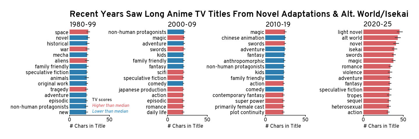

This again illustrates how much longer anime titles have gotten. While certain titles have been consistently appearing in the top across the years (e.g. magic nd swords), in recent years, titles adapted from noves, especially light novels, and titles about alternative worlds (including Isekai) have jumped to the top of the list.

Let’s further visualize the top 5 in 2020-2025 and look back in time to see how much they have gotten longer. It really does seem that the trend has been much more accelerated in the recent 5 years for them.

n_select = 5
select_tags = (
    tags_vdf.sort_values(vis_by)
    .query('period == "2020-25"')
    .tail(n_select)['tag'].unique()
)

tags_sdf = (
    tags_df.explode('tags')
    .rename(columns={'tags':'tag'})
    .replace({'tag': renamed_tags})
    .query('tag in @select_tags')
)

tags_svdf = pd.concat([
    (
        tags_sdf.value_counts(['period','tag'])
        .to_frame('# Titles')
        .melt(ignore_index=False)
        .reset_index()
    ),
    (
        tags_sdf.filter(['period','tag','num_chars'])
        .rename(columns={'num_chars':'value'})
        .assign(variable='# Characters in Title')
    )
], ignore_index=True) 
tags_svdf

g = sns.catplot(
    tags_svdf,
    x='value',
    y='tag',
    hue='period',
    kind='bar',
    col='variable',
    palette=sns.blend_palette(
        # ['#fff0f3', '#E94B50'], 
        ['#e3f2fd','#1982C4'],
        tags_svdf['period'].nunique()
    ),
    edgecolor='k',
    sharex=False,
    aspect=0.9,
    height=4.4,
    legend_out=False,
)
g.set_xlabels('')
g.set_ylabels('')
g.set_titles('{col_name}', size=22, ha='left', x=0)
g.tick_params(axis='y',length=0)
[ax.set_xlim([-2, None]) for ax in g.axes.flat]
g.despine(trim=True, offset=10, left=True)
sns.move_legend(
    g, "lower center",
    bbox_to_anchor=(.5, 0.15), 
    title='Time period', 
    edgecolor='k',
    title_fontsize=15,
    fontsize=14,
)

g.fig.suptitle(
    'Extreme Lengthening Was Very Recent',
    x=0.175, y=0.97, ha='left',
    fontweight='bold', fontsize=26,    
)
g.tight_layout(w_pad=4)

plt.savefig('figures/top5-recent.svg')
plt.savefig('figures/top5-recent.png')