Visualization: Are more movies set in the future or the past?#
Motivation#
I was curious about the balance between media set in the future vs movies set in the past. Luckily, people on Wikipedia have tagged movies both for when they are produced/released, as well as whether they are set in certain years, decades or centuries.
For example, Category:Films_set_in_1945 contains list of movies set in 1945, while Category:2022_films contains list of movies from 2022.
Obtain data#
The data are scraped from Wikipedia using category pages.
The produced years are from Category:Films_by_year.
The set-in years are from 3 categories:
Category:Films_by_century_of_settingCategory:Films_by_decade_of_settingCategory:Films_by_year_of_setting
See the scrape.ipynb notebook for more information.
Import modules#
Show code cell source
import os, re, pickle, time
import numpy as np
import pandas as pd

import matplotlib.pyplot as plt
from matplotlib import rcParams
import seaborn as sns
Show code cell source
# plot configs
rcParams['font.family'] = 'Overpass Nerd Font'
rcParams['font.size'] = 18
rcParams['axes.titlesize'] = 20
rcParams['axes.labelsize'] = 18
rcParams['axes.linewidth'] = 1.5
rcParams['lines.linewidth'] = 1.5
rcParams['lines.markersize'] = 20
rcParams['patch.linewidth'] = 1.5
rcParams['xtick.labelsize'] = 18
rcParams['ytick.labelsize'] = 18
rcParams['xtick.major.width'] = 2
rcParams['xtick.minor.width'] = 2
rcParams['ytick.major.width'] = 2
rcParams['ytick.minor.width'] = 2
rcParams['savefig.dpi'] = 200
rcParams['savefig.transparent'] = False
rcParams['savefig.facecolor'] = 'white'
rcParams['savefig.format'] = 'svg'
rcParams['savefig.pad_inches'] = 0.5
rcParams['savefig.bbox'] = 'tight'
Load data#
data_path = 'data/films_set_in_and_produced.csv'
df = pd.read_csv(data_path)
df
| pageid | title | source_year_setin | year_produced | year_setin | year_setin_type | |
|---|---|---|---|---|---|---|
| 0 | 3217 | Army of Darkness | 13th | 1992 | 1200 | century |
| 1 | 3333 | The Birth of a Nation | 1860s | 1915 | 1860 | decade |
| 2 | 3333 | The Birth of a Nation | 19th | 1915 | 1800 | century |
| 3 | 3333 | The Birth of a Nation | 1870s | 1915 | 1870 | decade |
| 4 | 3746 | Blade Runner | 2019 | 1982 | 2019 | year |
| ... | ... | ... | ... | ... | ... | ... |
| 20150 | 74597836 | The Sacrifice Game | 1971 | 2023 | 1971 | year |
| 20151 | 74607682 | Joachim and the Apocalypse | 12th | 2023 | 1100 | century |
| 20152 | 74612478 | The Kitchen (2023 film) | 2040s | 2023 | 2040 | decade |
| 20153 | 74619750 | Jailer (2023 Malayalam film) | 1950s | 2023 | 1950 | decade |
| 20154 | 74621258 | Robot Dreams (film) | 1980s | 2023 | 1980 | decade |
20155 rows × 6 columns
Brief notes on data#
It is intuitive that a movie can be set in multiple years.
But, a movie entry (by pageid) can be appear in multiple Wikipedia categories ABCD films. Technically they’re not always produced in such years.
As I understand there may be different scenarios as to how this happens, for example release dates or an entry is a TV series.
df.query('pageid == 67231914')
| pageid | title | source_year_setin | year_produced | year_setin | year_setin_type | |
|---|---|---|---|---|---|---|
| 19286 | 67231914 | Edge of the World (2021 film) | 19th | 2021 | 1800 | century |
| 19287 | 67231914 | Edge of the World (2021 film) | 19th | 2023 | 1800 | century |
For example, Edge of the World (2021 film) belongs to both Category: 2021 films and Category: 2023 films. The Wikipedia page says
Edge of the World was released in the US […] on 4 June 2021, […] then in the UK […] on 21 June 2021.
In Malaysia and Brunei, the film has been slated as Rajah in the countries and scheduled on 9 March 2023 in cinemas.
Similarly, the Wikipedia box says
Release dates
4 June 2021 (US)
9 March 2023 (Malaysia and Brunei)
So this is due to different release dates.
df.query('pageid == 6819660')['year_produced'].unique()
array([1967, 1968, 1969, 1970, 1971, 1973])
Another example is Adventures of Mowgli, with 6 different years for production/release. This is not entirely like the above example with similar content and different release dates, but actually 5 different contents (1967-1971) and then later combined into one content released in 1973.
Adventures of Mowgli (Russian: Маугли; also spelled Maugli) is an animated feature-length story originally released as five animated shorts of about 20 minutes each between 1967 and 1971 in the Soviet Union. […]
In 1973, the five films were combined into a single 96-minute feature film.
Hence, take note that year_produced should be taken with a jitter of a few years in mind in some cases. Plus, it is not correct that is is produced, it may be a combination of production and release, maybe even (re)distribution.
For simplicity, I will not consider movie titles and ignore this for the time being, and instead analyze all pairs of (year_produced, year_setin).
Get time difference#
This is to calculate the time difference between year_setin and year_produced, with consideration of units.
If the time difference is positive, the movie is set in the future of the time that it is produced/released, e.g. post-apocalyptic movies.
If it is negative, the movie is set in the past, e.g. war movies.
df['year_diff'] = df['year_setin'] - df['year_produced']
df['diff_unit'] = df['year_setin_type']
df['num_years'] = df['diff_unit'].map({'century': 100, 'decade': 10, 'year': 1})
df['time_diff'] = df['year_diff'] / df['num_years']
df
| pageid | title | source_year_setin | year_produced | year_setin | year_setin_type | year_diff | diff_unit | num_years | time_diff | |
|---|---|---|---|---|---|---|---|---|---|---|
| 0 | 3217 | Army of Darkness | 13th | 1992 | 1200 | century | -792 | century | 100 | -7.92 |
| 1 | 3333 | The Birth of a Nation | 1860s | 1915 | 1860 | decade | -55 | decade | 10 | -5.50 |
| 2 | 3333 | The Birth of a Nation | 19th | 1915 | 1800 | century | -115 | century | 100 | -1.15 |
| 3 | 3333 | The Birth of a Nation | 1870s | 1915 | 1870 | decade | -45 | decade | 10 | -4.50 |
| 4 | 3746 | Blade Runner | 2019 | 1982 | 2019 | year | 37 | year | 1 | 37.00 |
| ... | ... | ... | ... | ... | ... | ... | ... | ... | ... | ... |
| 20150 | 74597836 | The Sacrifice Game | 1971 | 2023 | 1971 | year | -52 | year | 1 | -52.00 |
| 20151 | 74607682 | Joachim and the Apocalypse | 12th | 2023 | 1100 | century | -923 | century | 100 | -9.23 |
| 20152 | 74612478 | The Kitchen (2023 film) | 2040s | 2023 | 2040 | decade | 17 | decade | 10 | 1.70 |
| 20153 | 74619750 | Jailer (2023 Malayalam film) | 1950s | 2023 | 1950 | decade | -73 | decade | 10 | -7.30 |
| 20154 | 74621258 | Robot Dreams (film) | 1980s | 2023 | 1980 | decade | -43 | decade | 10 | -4.30 |
20155 rows × 10 columns
Visualization#
Plot distribution of years set-in#
Show code cell source
plt.figure(figsize=(18,5))

count_offset = 15

select_periods = {
    'US Civil War': [1861, 1865],
    'World War I': [1914, 1918],
    'World War II': [1939, 1945],
}

select_years = {
    1969: 'Apollo 11\nMoon Landing',
    1999: 'before Y2K',
    2012: 'defunct apocalypse',
    2023: 'present year'
}

select_year_list = list(select_years.keys())

df_year_target = df.query('year_setin_type == "year"')

select_counts = (
    df_year_target
    .query('year_setin in @select_year_list')
    .value_counts('year_setin')
    .to_frame('count')
    .join(
        pd.Series(select_years).to_frame('desc'),
        how='outer'
    )
    .reset_index()
    .rename(columns={'index': 'year_setin'})
)

select_counts['count_offset'] = select_counts['count'] + count_offset


sns.histplot(
    df_year_target.query('year_setin > 1800 and year_setin < 2050'),
    x='year_setin',
    discrete=True,
    element='step',
    color='k',
    edgecolor='none',
    alpha=0.1
)


sns.scatterplot(
    select_counts,
    x='year_setin',
    y='count_offset',
    c='#12a4b6',
    s=25,
    marker='o',
    edgecolor='none'
)

for _, r in select_counts.iterrows():
    t_ha = 'left'
    t_va = 'center'
    t_yr = r['year_setin']
    c_os = r['count_offset']
    desc = r['desc']
    if pd.isna(desc):
        continue
    desc = f"{t_yr} ({desc})"

    x_text = t_yr + 2
    y_text = c_os

    if t_yr == 1969:
        # to avoid blocking
        x_text = t_yr
        y_text = c_os + 10
        t_ha='center'
        t_va='bottom'

    plt.text(
        x_text, y_text, desc,
        fontdict=dict(
            size=15,
            ha=t_ha,
            va=t_va
        )
    )

for desc, (y0, ye) in select_periods.items():
    c_os = (
        df_year_target
        .query('year_setin >= @y0 and year_setin <= @ye')
        .value_counts('year_setin')
        .max()
    ) + count_offset

    plt.plot(
        [y0-0.5,ye+0.5], [c_os, c_os],
        color='#12a4b6', lw=2,
        marker='.', markersize=10
    )

    desc = f'{desc}\n({y0} - {ye})'

    plt.text(
        (y0 + ye)/2, c_os + count_offset/2, desc,
        fontdict=dict(
            size=15,
            ha='center',
            va='bottom',
        )
    )

plt.xlabel('Years that movies are set in (restricted to 1800 - 2050, set-in type = "year")')
plt.ylabel('Number of movies')
plt.suptitle('Distribution of years that movies are set in', fontsize=20)

sns.despine(trim=True, offset=10)
plt.tight_layout()

plt.savefig('figures/distrib-years-setin.pdf')
plt.savefig('figures/distrib-years-setin.png')
(
    df_year_target
    .query('year_setin in [1944,1945]')
    .value_counts('year_setin')
)
year_setin
1944    195
1945    167
dtype: int64
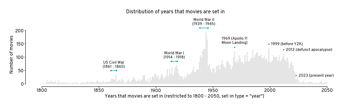
Many movies tend to be set in war periods, especially World War II (1939 - 1945). Interesting, there are more movies set in 1944 (195 movies) than in 1945 (167 movies). Not sure why.
Additionally, besides war periods, some notable events are annotated in the distribution and have high peaks as well, such as:
1969: Apollo 11 Moon Landing
1999: the year before Y2K. I annotated as such because I suspect this is why there’s a high peak in 1999 instead of 2000.
2012: the supposed end-of-the-world
Plot time difference between set-in and produced#
Show code cell source
plt.figure(figsize=(18, 5))

setin_types = ['year', 'decade', 'century']
t_range = [1880, 2030]

limits = dict(
    year = dict(x1=t_range, x2=[-0.001,0.05], y=[-450, 150]),
    decade = dict(x1=t_range, x2=[-0.01,0.6], y=[-60, 20]),
    century = dict(x1=t_range, x2=[-0.01,0.6], y=[-30, 10]),
)

num_cols = len(setin_types)

for i, st in enumerate(setin_types):
    ax = plt.subplot(1, num_cols, i+1)
    df_st = df.query('year_setin_type == @st')

    sns.scatterplot(
        df_st,
        x = 'year_produced',
        y = 'time_diff',
        s = 30,
        c = 'k',
        alpha = 0.02,
        edgecolor = 'none',
        ax = ax
    )

    ax.hlines(0, *t_range, colors='k', linestyles=':', alpha=0.4)

    ax.set_xlim(limits[st]['x1'])
    ax.set_ylim(limits[st]['y'])

    ax_twin = ax.twiny()
    sns.kdeplot(
        df_st,
        y = 'time_diff',
        color = 'k',
        ax = ax_twin
    )

    scale_bar_y = limits[st]['y'][-1]/2
    scale_bar_x = [abs(limits[st]['x2'][0])*2, limits[st]['x2'][1]/10]
    scale_bar_x[1] += scale_bar_x[0]
    ax_twin.hlines(scale_bar_y, *scale_bar_x, colors='k')
    ax_twin.text(
        sum(scale_bar_x)/2,
        scale_bar_y * 1.1,
        'density\n%.3f' %(scale_bar_x[1] - scale_bar_x[0]),
        fontdict=dict(size=12, ha='center', va='bottom', style='italic')
    )

    ax_twin.set_xlim(limits[st]['x2'])
    ax_twin.set_xlabel(None)
    ax_twin.set_xticks([])

    ax.set_xlabel('Production (or release) year')
    ax.set_ylabel(f'# {st}')
    ax.set_title(f'Set in {st}')

plt.suptitle(
    'Time difference between set-in years and production years',
    fontsize=22
)

sns.despine(trim=True)
plt.tight_layout()

plt.savefig('figures/produced-vs-timediff.pdf')
plt.savefig('figures/produced-vs-timediff.png')
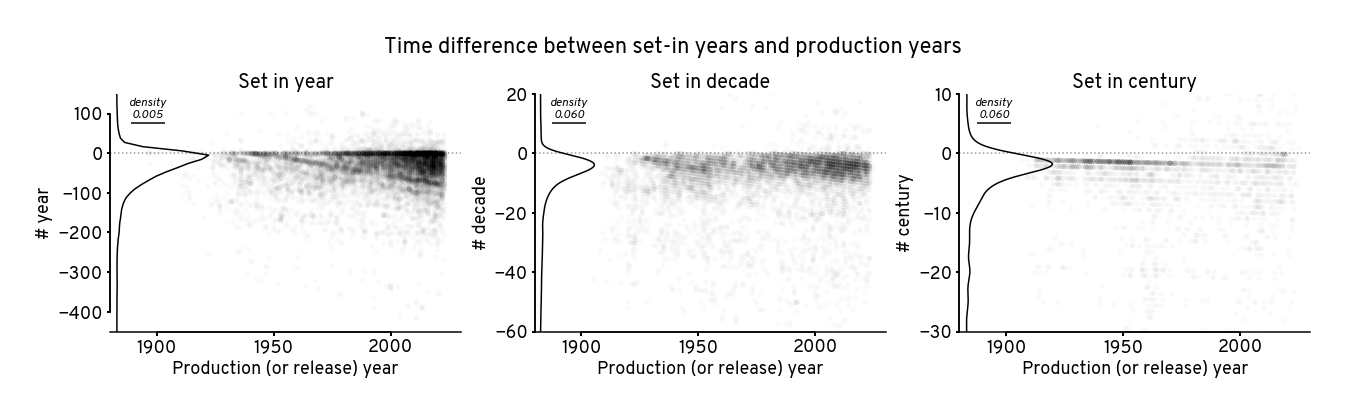
Considerable number of movies are set in the past, even more so than setting in the present. The tail towards the past is much heavier than it is for the future.